The first time you run an atmospheric model like OpenIFS in single precision (SP, 32-bit float), the global mass diagnostics will probably give you a scare.
In our recent 90-day benchmark runs with ECMWF OpenIFS CY48R1.1 on the octahedral reduced Gaussian grid (TCo79L91, 1-hour time step), the total global atmospheric $\mathrm{CO}_2$ mass in SP ended up differing from our Double Precision (DP) reference run by roughly 2,000 Tg (about 0.06% of the entire atmospheric inventory).
When you see that number, the natural reaction in the group is almost always: our advection scheme has a serious mass leak in single precision.
Except it doesn’t. When we instrumented the code to track the mass budget term-by-term, we discovered that over 99.5% of that 2,000 Tg spread wasn’t transport leakage at all—it was chaotic weather divergence.
Here is what is actually going on mathematically, why evaluating total mass alone is a trap, and how we used stochastic rounding to eliminate the true numerical truncation drift.
1. Don’t Look at Total Mass Alone: Decomposing the Budget
If you only look at the total mass curve $M(t)$, you can’t tell whether mass vanished into numerical thin air or was absorbed by the ocean.
To solve this, we hooked into the diagnostic tendencies in chem_massdia.F90 to break the net atmospheric tracer change into four distinct terms:
$$\Delta M(t) = E_{\text{emis}}(t) + S_{\text{chem/sfc}}(t) + \Delta M_{\text{transport}}(t) + \text{Residual}(t)$$
- Prescribed Emissions ($E_{\text{emis}}$): Surface emissions and 3D aircraft injections ($+10{,}417.5\text{ Tg}$ over 90 days). Because this is read from input files, it is bit-identical across all DP and SP runs.
- Interactive Surface Sinks ($S_{\text{chem/sfc}}$): Dynamic ocean gas exchange and biospheric uptake, where ocean flux scales with surface wind speed and temperature ($F_{\text{ocean}} \propto k(U_{10}^2, T_s) \cdot \Delta p\mathrm{CO}_2$).
- Pure Transport Error ($\Delta M_{\text{transport}}$): The cumulative corrections applied by the advective mass fixer ($\sum \delta M_{\text{fixer}}$).
- Discretization Residual: Coordinate mapping differences between spectral dynamics and physical Gaussian grid points.
2. What the 90-Day Diagnostics Reveal
Here is the 4-panel diagnostic tracking all 90 days across 5 different model configurations:
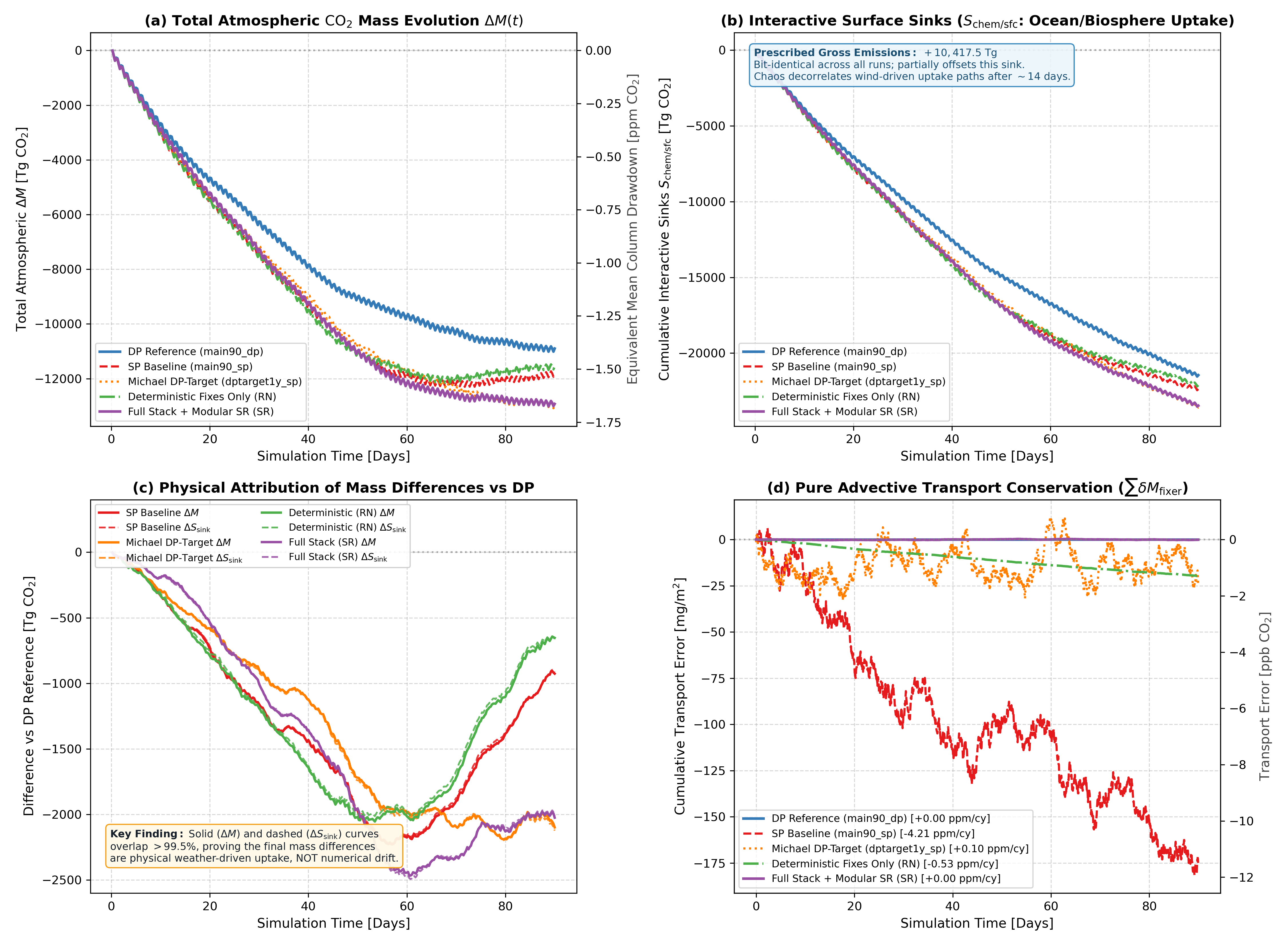
Take a close look at Panel (c):
- The solid line is the total mass discrepancy relative to the DP reference run ($\Delta M_{\text{SP}} - \Delta M_{\text{DP}}$).
- The dashed line is the surface sink discrepancy ($\Delta S_{\text{chem,SP}} - \Delta S_{\text{chem,DP}}$).
The solid and dashed curves sit right on top of each other (>99.5% match across all 90 days).
Why? Because during the first 10–14 days (the deterministic predictability window), SP and DP track identically. But once the atmosphere decorrelates chaotically, storm tracks shift slightly between the two runs. Different storm tracks mean different 10-meter wind speeds ($U_{10}$) over the ocean, which directly changes the integrated gas uptake.
The model isn’t leaking mass; it is simply simulating two slightly different, equally valid weather paths.
3. The True Leak: Truncation Bias in the Mass Fixer
That said, single precision does have a real numerical error—it is just subtle. It shows up in Panel (d), which isolates the cumulative mass fixer corrections ($\sum \delta M_{\text{fixer}}$):
| Simulation Run | Total Atmospheric $\Delta M$ | Interactive Sinks ($S_{\text{chem}}$) | Fixer Error ($\sum \delta M$) | Secular Drift Rate |
|---|---|---|---|---|
DP Reference (dp_ref) | $-10{,}898.9\text{ Tg}$ | $-21{,}456.4\text{ Tg}$ | $+0.000\text{ Tg}$ ($0.0\text{ }\mu\text{g/m}^2$) | $+0.00\text{ ppm/century}$ |
SP Baseline (sp_base) | $-11{,}825.3\text{ Tg}$ | $-22{,}373.7\text{ Tg}$ | $-89.262\text{ Tg}$ ($-175.0\text{ mg/m}^2$) | $-4.21\text{ ppm/century}$ |
| Deterministic Fixes Only (RN) | $-11{,}552.3\text{ Tg}$ | $-22{,}116.2\text{ Tg}$ | $-10.014\text{ Tg}$ ($-19.6\text{ mg/m}^2$) | $-0.53\text{ ppm/century}$ |
| Full Stack + Stochastic Rounding (SR) | $-12{,}923.8\text{ Tg}$ | $-23{,}469.8\text{ Tg}$ | $-0.020\text{ Tg}$ ($-39\text{ }\mu\text{g/m}^2$) | $+0.00\text{ ppm/century}$ |
In the standard single-precision code, IEEE 754 Round-to-Nearest (RN) creates a tiny negative truncation bias at every grid point and time step ($\mathbb{E}[e] \neq 0$). Accumulated over tens of millions of grid points and thousands of time steps, it adds up to a steady drift of $-4.21\text{ ppm per century}$. For long climate runs, that’s a problem.
4. Fixing It with Stochastic Rounding
We don’t want to run the whole model in double precision—that would double memory traffic and throw away single-precision performance gains on modern supercomputers.
Instead, we implemented a SIMD-friendly Stochastic Rounding (SR) kernel inside the quasi-monotone fixer (qmfixer.F90).
The Basic Idea
When downcasting the exact double-precision target mass $y = Z_{\text{FAC}} \cdot q$ to single precision $x$:
- $y$ falls between $x$ and its nearest float neighbor $x_{\text{adj}} = \text{NEAREST}(x, \Delta)$.
- The distance between them is 1 Unit in the Last Place: $\delta = |x_{\text{adj}} - x|$.
- Instead of always picking the closest neighbor, we choose $x_{\text{adj}}$ with probability $p = |\Delta| / \delta$, and keep $x$ otherwise.
Because $\mathbb{E}[\hat{x}] = y$, the expected error at each step is strictly zero. Testing $U \cdot \delta < |\Delta|$ (with $U \sim \text{Uniform}(0, 1)$) lets us evaluate this without any floating-point division:
IF (KIND(1.0_JPRB) == KIND(1.0_JPRD)) THEN
  ! Double Precision: compile-time branch elimination, zero overhead
  !$OMP PARALLEL DO SCHEDULE(STATIC) PRIVATE(...)
  DO JKGLO=1,NGPTOT,NPROMA
    ...
    PGFLT1(JROF,JLEV,YCOMP(JGFL)%MP1,IBL) = &
      REAL(ZFAC_DP(JFIX) * DBLE(PGFLT1(JROF,JLEV,YCOMP(JGFL)%MP1,IBL)), KIND=JPRB)
  ENDDO
  !$OMP END PARALLEL DO
ELSE
  ! Single Precision: Stochastic Rounding to kill secular drift
  !$OMP PARALLEL DO SCHEDULE(STATIC) PRIVATE(...)
  DO JKGLO=1,NGPTOT,NPROMA
    ...
    ! Fast hash PRNG evaluated per grid cell
    IF (ZRAND * ZSTEP_DP < ABS(ZDIFF_DP)) THEN
      PGFLT1(JROF,JLEV,YCOMP(JGFL)%MP1,IBL) = ZNEXT_SP
    ELSE
      PGFLT1(JROF,JLEV,YCOMP(JGFL)%MP1,IBL) = ZVAL_SP
    ENDIF
  ENDDO
  !$OMP END PARALLEL DO
ENDIF
What This Gives Us
- Zero DP Overhead: When running in DP, the compiler eliminates the
ELSEbranch entirely. No extra instructions, no performance impact. - From Linear Drift to a Random Walk: By making the rounding unbiased, truncation error stops accumulating linearly as $O(N)$ and turns into a bounded random walk $O(\sqrt{N})$.
- Double Precision Accuracy: Cumulative transport mass loss dropped from $-89.3\text{ Tg}$ down to $-0.02\text{ Tg}$ ($-39\ \mu\text{g/m}^2$). The secular drift rate is now $+0.00\text{ ppm/century}$, matching DP precision while keeping single precision speed.